This is more in the nature of notes for a proper post, but I'll put it here. If you want to read some sense, check James Annan: still flapping. If you want some nonsense, then follow the link therein to RP :-)
But first: something completely different:
So, I took HadAM3 (64 bit version) and did two runs: one standard, and one where I perturbed the surface pressure at a single grid point (I forget where: somewhere in the Arctic I think) by a tiny amount (1e-10, or was it 1e-12?).
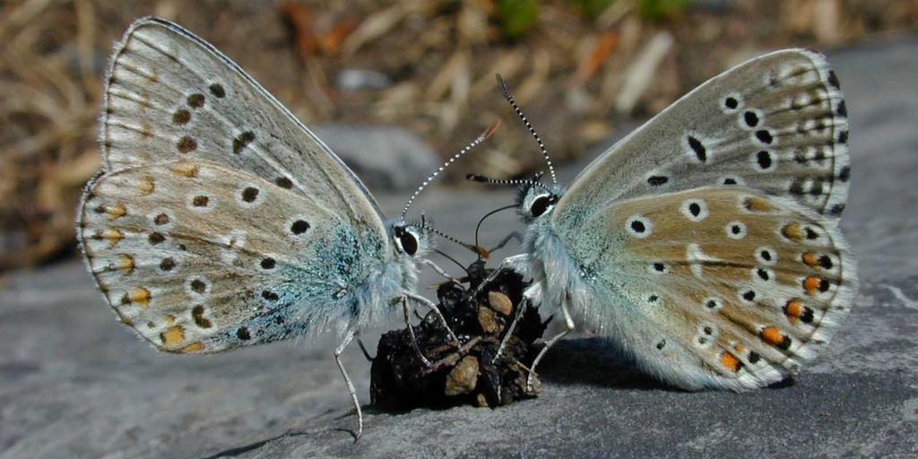
The graph below shows the growth in global-mean area-weighted RMS of the difference of the MSLP field between the two runs:
The x-axis is time in days (48 timesteps per day): 0-5 (top); then 0-15 (mid); then 0-89 (bottom). By day about 25, and definitely by day 60, the difference between the runs has saturated: their weather is totally different, so no further growth in RMS occurs. The 5-10 day oscillations in the last month are, I think, what you'd expect to see from weather evolution.
The y-axis is in Pascals. 100 Pascals is an hPa, ie 1 mb. Standard weather charts tend to plot pressure in contours of 4 hPa, so in real weather terms the diffs are sort-of negligible out to about day 15 (although this is a global value, so locally there will probably be bigger values).
There are clearly different phases in the difference growth. After day 25-ish there is a slow rise to saturation. From day about 10 to about 25 there is exponential growth. From day 2 to 10 ish there isn't much growth. And from the start to about day 1 there is another exponential phase.
If you look carefully, you'll see that the diff appears to be zero for the first few timesteps. This isn't really true. But the model output (as opposed to its internal variables) has been converted from 64 to 32 bit floats; and the difference is identically zero at 32 bit (but not 64).
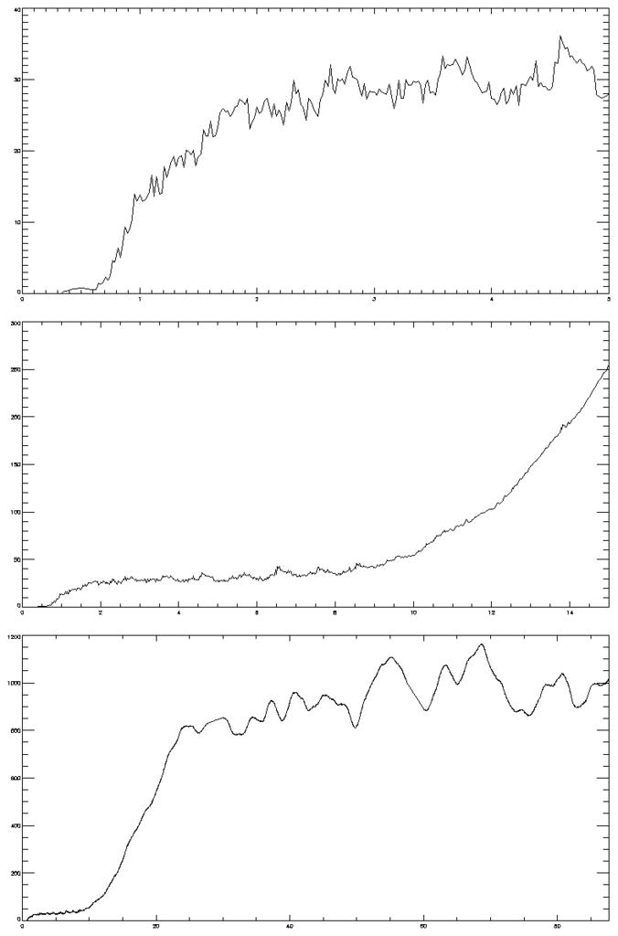
Meanwhile, its interesting to look at the pattern of the diffs.

The top pic is about day 4 (in the not-much-happening phase). The middle, day 15 (in the exp growth). The bottom, day 31 (saturated). Note that the pics have a different contour interval. By days 15/31 we're into "real meteorology" and hence the MSLP field is most different in extratropics, as it always is (its tropical dynamics, folks). The fact that the biggest diffs on day 4 are in the tropics (is this convection being jigged?) says we're in a different regime, but I'm a bit unsure.
So there we are for now. Over to you, James.
[The original post was oct 15. I've updated the timestamp.
Update: I've been playing with the timestep-dependence of this. In the pic below, the black line (solid) is run "a" (std) minus run "b" (small pert); black dashed is a-c, where "c" is a different small pert. Blue is the same but for with all three runs done at 1/2 the timestep. Red also, but for 1/4 the timestep. The std timestep is half hour. There are plenty of caveats here: firstly, that this is really only playing. Secondly, that all I did was change the value marked timestep (actually, the value marked "steps per period" from 48 to 96 to 192) without checking that anything was going hideously wrong elsewhere. Thirdly, that if you compare this to the previous plot you'll notice that its spikier: because its 6-h data (instantaneous) not timestep data. Fourthly, that even if nothing is going hideously wrong, changing the timestep does give a different model (is the climatology the same? I don't know. Maybe). For example, the atmos is fourier-filtered at the poles for CFL reasons. A smaller timestep means less area if filtered.
Also: to answer JA's q: does the pert grow one-box-per-timestep (ie, unphysically?). Well no. It grows faster than that, because, ha ha, the perturbation is within the filtering zone so it grows into the entire northern polar cap within a few timesteps.
But: the plot below shows that the initial growth is *slower* with smaller timestep (well even this is complex: the 1/2 timestep run grows faster up to day 1; but then the "plateau" level reached by it is lower between days 2 and 10; and the 1/4 timestep plateau is lower again. Does this mean that a very very small timestep (arguably, as physical reality has?) would have a very low (zero?) plateau? I must try some even shorter timesteps. BUT then you end up in territory where the model was never designed for and it becomes rather dodgy.

Having 3 different runs at each timestep (more would be nice of course) allows you to see that during the day 15-30 growth phase, the timestep doesn't matter. But earlier, it clearly does.
Curious. I wonder what it means...
ps: sorry James. I'll get back to it :-(
20 comments:
Peter: Of course you're right: there is only one world. To make the butterfly effect thingy work, we have to do a thought experiment: what if we had a copy world, identical except for one butterfly's flap.
All of these things, if any one were different, would send the *weather* off on a different course. But the climate would be unchanged.
The two phase growth is nice. If I remember the NWP stuff correctly, the initial growth in the perturbation is due to local convective instability, which takes some time to influence the mesoscale. This is exactly why NWP centres look for meteorologically interesting perturbations (for ensemble forecasts) rather than just adding random noise. In the infinitesimal limit, it is the convective instability that grows fastest, so searching for perturbations requires some careful treatment when singular vector methods are used.
I'm a little surprised that it kicks off so quickly on the global scale. I wonder if the pertubation spreads at a meteorologically plausible rate, or is it diffusing at a "numerical" rate of one grid point per time step? Anyway, it all looks very pretty.
So how big are your grids/timesteps and how many butterfly wing flaps does it take to equal the pressure pertubation you put in.
Grid is 2.5 (lat) x 3.75 (long), ie about 300 km. The perturbation was to change the surface pressure frm 99424.80078124999 to 99424.80078125009 at a certain point. So I could have made it smaller, and perhaps will.
How that relates to butterfly-flaps I'm not sure. As far as the model is concerned, it doesn't matter I think: the behaviour is about scale-indep.
Just to make sure: HadAM3 (64 bit version) gives bit-identical runs when started with the same initial conditions on the hardware that you're using?
Cr - glad you liked it. There may be more to come but I don't promise.
Arun: yes, its repeatable (and indeed restartable in mid run too).
Belette - Very interesting, but the graphs were too small for me to read. Also, what are the three different top graphs? Is there any way you could show this with some legends, on a slightly larger scale?
CIP - ah; are the graphs still too small when you click on them? The top one is 3 different time periods (you can tell that if you look closely at the shape of the graph).
On the first one, the top is days 0-5, and the y axis is 0-40. The mid one is to day 15, and the y axis to 300. The bottom one is to day 90, and the y axis to 1200 (Pa).
I may get round to redrawing them tonight.
I have pointed this out in James's Blog, but it is being ignored so I am reposting my idea here, where it is more appropriate.
IMHO, your experiment has a flaw which can be easily corrected. By alterering the pressure in only one cell your are contravening the law of conservation of energy. The air pressure at a point on the surface of the Earth is determined by the weight of the column of air above it. It you reduce the pressure, then you are in effect altering the mass of air in the column. In the case of a butterfly flapping its wings global mass remains constant. To simulate a butterfly's flap you need to alter the pressure in two cells with equal and opposite effect. In that case, with the mass effectively being rtransfered from on cell to another, it would be possible to see if the model converged, or diverged as a result of the butterfly's flap, rather than due to a change in mass.
Very curious to know the result,
Cheers, Alastair.
Hi Alistair. I see your point, but I can tell you the result without doing it: it will simply generate a different trajectory. Energy conservation down to that level is, I think, not important. But... I might get round to trying it.
I'll paste in here a quote from Raymond Arritt to sci.env, which helps (perhaps):
>The chaos argument isn't that one particular small vortex grows into
>another particular large vortex. Rather, the initial disturbance
>creates small changes to the atmosphere that cause it to evolve in a
>different way. The overall statistical properties of the system remain
>the same, but the specific events happen in a different way -- tornado
>alley is still tornado alley, and the tornados still happen mostly in
>the spring, but the individual storms don't happen in exactly the same
>place and time as if the butterfly hadn't flapped its wings.
OK, I did try it, it did make very little difference, as I predicted (hurrah, a prediction coming true...).
See it at: http://www.antarctica.ac.uk/met/wmc/butterfly-2.png if you like (the blue line is the new run).
Right! I had been thinking about the that experiment before I saw the result. It occured to me that if you put the second point diametrically opposite the first on the world stage, then the first point would behave in the same manner as it did in the first experiment, until eventually the effect of the second point had spread far enough for it to interfere with the first. By that time there would be no prospect of the two points giving the same result as no point.
OTOH if you placed the two points adjacent to each other, they could eliminate each others effect. If this elimination does happen, then there must be a maximum distance at which this elimination would happen, and let's call the locus of this distance in the phase space the edge of the basin of attraction. (The phase space in this case is in fact a physical distance! well virtual really.)
In your figure you have not labelled the axes, and so I am assuming that the x axis is in time steps of the model. I am also assuming that the y axis is the error distance of the first point from its value in the unperturbed run. If this is true then since the black line and the blue line diverge only after the tenth time step, am I correct in deducing that the two perturbing points were placed 10 points apart?
If so, it would be interesting to see what would happen it the points were placed closer together. Judging by the shape of the black line which suddenly "takes off" at around ten steps, it could be that ten points is the distance to the edge of the basin of attraction!
So I have two questions: why does the the black line (and the blue line) take off after 10 timesteps, and why do the blue and black lines coincide for ten time steps, and is the ten timesteps in both my questions a coincidence?
Hoping you can find time to answer these questions,
Cheers, Alastair.
Alistair: I did put the perturbation point next to each other. As I expected, they don't cancel.
The x axis is in days, just like the post days, not time steps.
The y axis is given in the post too. You just have to read it carefully.
The blue and black lines are non-identical immeadiately, but diverge obviously after 10 days. No, they aren't 10 pts apart.
Score 1 for my prediction ability but -1 for yours :-)
Fair enough, but I think you have miscalculated my score. I made two predictions; that the points were ten points apart, and if they were less than ten points they would not diverge. Since the second depends on the first I deserve double points for that one, and so my score should be -3!
The actual question was: "Predictability: Does the Flap of a Butterfly’s Wings in Brazil set off a Tornado in Texas?" See http://www.cmp.caltech.edu/~mcc/chaos_new/Lorenz.html so the answer seems to be yes.
That doesn't answer my two questions though :-(
Cheers, Alastair.
From my comment on sci.environment:
James Annan wrote:
>Well, they do not deal in momentum directly, but velocity and pressure.
>A small enough perturbation could in theory be rounded out, but we can
>always compile the model at higher precision, and as wmc already showed,
>in practice it tends to grow fairly rapidly due to convective instability:
>(the results are entirely routine and characteristic of small
>perturbations in GCMs)
I think your last comment says it all. "Perturbations in GCM's" are not the real world. How do you know for sure that the different trajectories are NOT due to the internal workings of the model, where there are numerous truncations and quantizations, such as the 48/day time step and the relatively
large grid size?
I think WMC should try the same experiment with a smaller grid and smaller time step and see if the difference between the two runs produces the same level of divergence with time. I suggest four cases, actually, one one with smaller grid, one with smaller grid and smaller time step, one with smaller grid, large time step but perturbed and last, one with both small grid, smaller time step
and perturbed.
ES
Your Wikipedia account will probably have to be disabled because you have violated the parole - for example on the page of Bjorn Lomborg. This hurts the Wikicommunity.
Wikipedians
Its Michael "no sense of history" Sirks! Hello and welcome, err, or are you? To be honest, no, you aren't really. Had any luck with JG or C yet, ho ho? [Please dont take this as an invitation to post further irrelevancies.]
Meanwhile: CR: yes: I agree, trying a tropical perturbations would be a good idea. Also because it would be out of the fourier filtering zone so watching the growth over the first few timesteps might be more interesting. Trying bigger/smaller perts is also an interesting idea. I *have* just tried it with 1/8 and 1/16th timesteps (so sloooooow) and the "first stage plateau" *doesn't* monotonically decline... which is good, I think.
But there are so many other things to try: for example, the convective code is called every timestep... but I could call it every 1/2 hour instead... doing this properly is a research project in itself, not an evening job!
Hi William!
If you want to simplify the work for Interpol, you may list your numerous crimes yourself at:
WMC investigation at Wikipedia
Have you written your last will yet? ;-)
All the best
Lubos
Ah Lubos, I take this as a confession of failure on your part: unable to stuff wiki with your POV by fair means, you resort to foul. But, my prediction is that wiki will shrug you off as it did before.
Post a Comment